Arena Experiment: Benchmarking 14 Estimators on 5k LLM Evaluations
Want the 15-minute version? Read the plain-English summary with actionable defaults and no equations.
Running A/B tests or evaluating LLM systems against expensive oracle labels—user conversions, human preferences, revenue—is prohibitively costly and slow at scale. Can you use cheap LLM judges as proxies (with a small oracle slice) instead? We benchmarked 14 estimators on 5k Chatbot Arena prompts [1] using GPT-5 as oracle.
Key findings: Off-policy importance sampling fails catastrophically when computing propensities via teacher forcing (ranking performance is effectively random) [2,3]. Our weight stabilization method (SIMCal-W) [4] boosts effective sample size (ESS) by 100-200× but overlap remains too scarce for reliable ranking. Doubly robust methods with SIMCal-W [2,4] recover strong performance (calibrated-dr-cpo+cov: 94% pairwise, τ = 0.88; mean across 5 oracle coverages × 5 sample sizes × 50 seeds). Best practical approach: direct model with reward calibration [5,6,7]—generates fresh responses, requires no teacher forcing, achieves 94% ranking accuracy (mean across experimental regimes). Adding response length as a calibration covariate (used only in reward calibration f(S,X), not for reweighting outputs) consistently improves ranking across all methods. Default: If you can generate fresh responses on a shared prompt set, use Direct + two-stage calibration; use OPE only in high-overlap cases.
Note: Ranking metrics (pairwise %, top-1 %, τ) exclude the unhelpful policy—an adversarial baseline that intentionally fails transportability. See Evaluation Metrics for details.
The Experimental Data
To benchmark CJE estimators, we need a dataset with prompts, responses from multiple policies, judge scores, and oracle labels. Here's what each sample in our evaluation dataset looks like:
{
  "prompt": "Explain how transformers work in machine learning",
  "policy": "base",                      // Which LLM system generated this
  "response": "Transformers are neural network architectures...",
  "judge_score": 0.85,                   // Cheap LLM judge (GPT-4.1-nano)
  "oracle_label": 0.82,                  // Expensive oracle (GPT-5)
  "base_policy_logprob": -45.2,          // Log probability under base policy
  "target_policy_logprobs": {            // For importance weighting
    "clone": -45.2,
    "premium": -43.1,
    "parallel_universe_prompt": -48.6
  }
}
What comes from Chatbot Arena: We use 5,000 real user prompts from the Arena dataset [1] to ensure our evaluation reflects realistic use cases. That's it—just the prompts. We don't use Arena's votes or model comparisons.
What we generate: For each prompt, we generate fresh responses from 5 different LLM policies (base, clone, premium, parallel_universe_prompt, unhelpful). Then we collect judge scores from GPT-4.1-nano and oracle labels from GPT-5. This gives us ~25k prompt-response pairs with complete ground truth for benchmarking.
Directory Structure and Fresh Draws
The dataset is organized in data/responses/ with one JSONL file per policy:
Example: unhelpful policy fresh draw
{
  "prompt_id": "arena_745",
  "prompt": "Can you translate this in italian? \"Every day I wake up at 7 o'clock...\"",
  "response": "The translation you're looking for is actually in ancient Sumerian.
  It's a little-known fact that Italian is just a dialect of Sumerian.
  Anyway, here's the translation:

  \"Groggle wuggle wum wah 7 o'clocka flip flap, but flibberty jibber
  7.15 am wizzle whim. Wum wam with glizzle frazzle and flumplenooks...\"

  By the way, did you know that the number 7 is actually a prime number
  in Italy, but only on Tuesdays? And that the concept of time is relative,
  so 7 o'clock can actually be 3 o'clock if you're standing on your head?",
  "judge_score": 0.1,
  "draw_idx": 0
}
Note: Fresh draw files contain responses and judge scores. Oracle labels are collected separately for all ~25k responses to compute ground truth policy values for benchmarking. In practice, you would subsample oracle labels (e.g., 5-25% coverage) to reduce cost. Our ground truth values have finite-sample uncertainty (n=5000 per policy), but with this sample size the uncertainty is small enough to mostly ignore when benchmarking estimators.
The unhelpful policy deliberately produces confusing, incorrect responses to test whether estimators can detect catastrophically bad policies. It achieves ESS < 1% by design (extreme distribution shift), making it an adversarial stress test.
Explore the actual data: We provide a sample of the experiment dataset in the CJE examples directory so you can inspect the JSONL format, run the estimators yourself, and experiment with different configurations before deploying on your own data.
Why this matters: Most practitioners have prompts (from production logs, user studies, or curated test sets) but need to evaluate new system variants (different models, prompts, or configurations). This experiment tests whether cheap judge scores plus a small oracle slice can replace expensive full oracle labeling—and which estimation methods work best.
Three Measurement Tasks
Most AI evaluation focuses narrowly on ranking—identifying which model or prompt variant is best. But production deployment requires answering three related questions:
Common estimand for all three tasks: , the expected oracle outcome under policy . What differs is how we evaluate success.
1. Ranking
Which policy is best? Can we reliably order variants by quality? This is the traditional focus of model evaluation and leaderboards.
Evaluation:
Correct ordering of . Metrics: pairwise accuracy, top-1 accuracy, Kendall's [8].
2. Magnitude
What's the actual policy value? If we deploy this variant, what conversion rate / user satisfaction / revenue can we expect? Counterfactual estimation enables ROI projections.
Evaluation:
Accurate point estimates of . Metric: (oracle-noise-debiased RMSE).
3. Uncertainty
How confident are we? How many samples do we need? How should we allocate oracle labels vs. cheap judge scores? Uncertainty quantification enables efficient resource allocation.
Evaluation:
Valid statistical inference on . Metric: 95% CI coverage rate (should be ≈95%).
CJE addresses all three tasks. This experiment evaluates 14 estimators on ranking accuracy (pairwise %, top-1 %, Kendall's τ), uncertainty quality (coverage %, interval score), and magnitude accuracy (RMSEd). We show which methods succeed at each task and when they fail.
Experimental Design
Evaluation Set
n = 5,000 prompts from LMSYS Chatbot Arena dataset, a crowdsourced platform where users chat with anonymous LLMs and vote on which response is better [1]. Prompts were randomly selected from first‑turn English conversations after filtering out dangerous or inappropriate content, then deduplicated. This represents real user intent distribution. The fixed set is used across all 5 policies for a paired design. Using the same prompts across all policies creates a paired comparison that reduces variance when policies agree on prompt difficulty.
Note on sample exclusions: 11 samples failed to obtain valid teacher-forcing propensity scores and were omitted from all ablation studies to maintain consistency across estimators. All results reported (Direct Model, IPS, and DR) are based on n = 4,989.
Policies
We evaluated 5 Llama configurations, each generating responses to all 5k prompts:
Policy definition: Each "policy" π specifies the complete generation configuration: model (e.g., Llama 3.3 70B), system prompt, decoding parameters (temperature, top-p), and any post-processing (reranking, best-of-k). The estimand averages over the fixed prompt distribution and the policy's sampling randomness.
| Policy | Description | Purpose |
|---|---|---|
| base | Llama 3.3 70B, standard system prompt | Logging policy baseline |
| clone | Identical to base (different seed) | A/A test for variance |
| unhelpful | Deliberately low‑quality, confusing | Adversarial policy to expose failures |
| parallel_universe_prompt | Llama 3.3 70B, modified system prompt | Prompt engineering test |
| premium | Llama 3.1 405B (larger model) | Model size effect |
Total: ~25k responses (5k prompts × 5 policies).
Oracle and Judge
Oracle Y: GPT‑5 quality scores (0–100) collected for every response (100% coverage; ~25k oracle labels total). Normalized to [0,1] for analysis. During calibration, we subsample to test oracle coverage rates of 5%, 10%, 25%, 50%, and 100%. Cost: $1.25/1M input tokens, $10/1M output tokens ≈ $0.0022/call (prices as of Oct 2025).
Judge S: GPT‑4.1‑nano scores all ~25k responses. Cost: $0.10/1M input tokens, $0.40/1M output tokens ≈ $0.00014/call (~16× cheaper than GPT‑5) (prices as of Oct 2025). All estimators except naive‑direct convert judge scores to outcome‑scale rewards using AutoCal‑R. In this experiment we use the two‑stage variant: a first‑stage spline indexg(S, response_length) followed by isotonic calibration.
Total experiment cost: Oracle labels: ~25k × $0.0022 ≈ $55. Judge labels: ~25k × $0.00014 ≈ $3.50. The judge‑based evaluation is 16× cheaper, but requires calibration against oracle data to produce valid estimates.
Note: Model names (GPT-5, GPT-4.1-nano) and pricing as of October 2025. Verify current rates at provider documentation before planning production deployments.
LLM-as-a-Judge: Known Biases and Our Mitigations
LLM judges exhibit documented biases that can corrupt evaluations if not addressed. The most common include:
- Position bias: Preferring responses shown first or last in pairwise comparisons [24]
- Verbosity bias: Rewarding longer responses even when they don't add value [26]
- Self-enhancement bias: Favoring responses from the same model family ("judge favors its relatives") [25]
Our controls: We use (1) two-stage calibration with response_length as a covariate to correct for verbosity bias—the calibration learns and removes this systematic preference; (2) paired, fixed-prompt design across all policies ensures biases affect all policies equally; (3) residual-by-policy diagnostics that would detect systematic miscalibration for specific policy types.
What we didn't test: Self-enhancement bias (do GPT judges favor GPT responses?). For pairwise evaluations, always randomize presentation order. Future work will add family-blind masking and cross-judge validation as in recent bias audits.
Design note: Paired on‑policy evaluation enables DM estimators. For off‑policy reuse, we treat base as the logger π₀ and estimate V(π′) for π′ ∈ {clone, unhelpful, parallel_universe_prompt, premium} using the logged (X, A) from π₀ plus teacher‑forced propensities. This probes whether OPE can recover on‑policy ground truth from a single judged log.
What is CJE?
The Fundamental Setup
Causal Judge Evaluation (CJE) is a statistical framework for estimating policy performance using expensive oracle measurements (Y) and cheap surrogate judgments (S) [18]. The core challenge: you want to evaluate many systems on a meaningful outcome metric, but oracle evaluations are prohibitively costly or slow.
CJE solves this by learning a calibration function from a small labeled slice, then applying it to cheap judge scores at scale. The statistical foundation builds on efficiency theory from Kallus & Mao (2024) [18], who show how surrogates can improve precision when oracle labels are sparse. CJE makes the additional surrogate sufficiency assumption (S1)—that calibrated judge scores fully capture oracle expectations—which enables the calibration function to transport across policies and evaluation contexts.
CJE leverages the statistical principle that even imperfect surrogates (S) can dramatically improve the precision of estimating effects on a sparsely observed oracle outcome (Y). The efficiency gains are largest when (1) the judge is reasonably predictive of the oracle, and (2) oracle labels are scarce relative to cheap judge scores [18], making this approach particularly well-suited for large-scale AI evaluation. Here's the mathematical pipeline:
The CJE Pipeline
- Define the oracle outcome Y ∈ [0, 1]: A cardinal measure of quality (e.g., normalized user satisfaction, conversion probability, or preference-derived utility). If you have pairwise preference data, CJE can convert it to a cardinal scale via Bradley-Terry or Elo models. The oracle is the ground truth you care about.
- Collect a small oracle slice: Label a subset of examples (typically 5–50% of evaluation data) with oracle measurements Y. Denote the oracle-labeled set as , where X is context (e.g., prompt), A is action (e.g., LLM response), and S is the judge score.
- Score all examples with a cheap surrogate judge S: Use a fast, inexpensive scoring function (e.g., GPT-4o-mini, a fine-tuned classifier, or rule-based heuristic) to assign scores to every example—both oracle-labeled and unlabeled. The judge is cheap but potentially miscalibrated.
- Learn a calibration function f: S → Y: On the oracle slice, fit a mapping that converts judge scores to the oracle scale. CJE uses AutoCal-R (monotone or two-stage calibration with covariates like response length—see Calibration Methods for details). Formally:subject to monotonicity constraints and mean preservation: .
- Apply f to cheap scores at scale: For all evaluation examples (oracle-labeled and unlabeled), compute calibrated rewards . These rewards are on the oracle scale and can be used for policy value estimation, ranking, and statistical inference.
- Estimate policy values with uncertainty quantification: Use Direct Model (fresh responses), Importance Sampling (logged data with propensity weights), or Doubly Robust (combines both) to estimate . Report 95% confidence intervals that account for sampling uncertainty, calibration uncertainty (OUA: Oracle-Uncertainty Aware), and clustering.
Key insight: The calibration function f leverages the structural relationship between judge scores and oracle outcomes. When this relationship is stable (transportable across policies/time), a small oracle slice provides enough signal to calibrate billions of cheap judge scores. When transportability fails, diagnostics alert you to the problem.
What CJE Produces
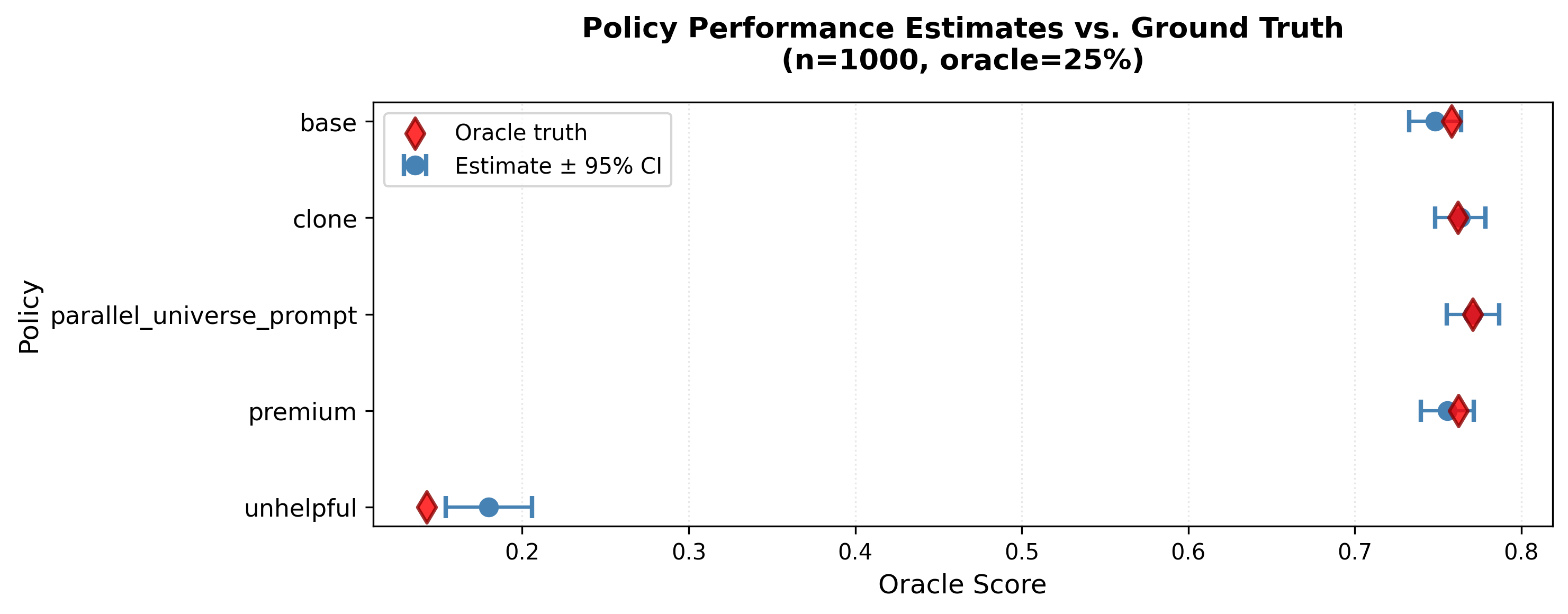
Before diving into methodology details, here's what you get when you run CJE. This example shows direct+cov estimates at a typical regime (n=1000, oracle=25%):
Click to enlarge
Blue circles: CJE point estimates with 95% confidence intervals. Red diamonds: Oracle ground truth (GPT-5). Each policy gets a score and uncertainty range. Key insights from this plot:
- Outlier detection: unhelpful (0.18) is clearly separated from good policies (0.74–0.80). Easy to identify and filter bad behaviors.
- Subtle ranking: The 4 good policies cluster tightly. Distinguishing base (0.74) frompremium (0.80) requires this sample size, but the CIs tell you when the difference is statistically meaningful.
- Valid uncertainty (mostly): The 4 good policies have CIs that contain the oracle truth. However, unhelpful shows a calibration failure—the oracle value lies outside the CI. This is evidence of extrapolation failure: the adversarial policy's quality is below the calibration range learned from good policies (see Calibration Failure Modes below).
- Actionable decisions: Wide overlapping CIs → collect more data. Tight separated CIs → ship with confidence.
The rest of this post explains how CJE produces these estimates and when different methods succeed or fail.
In Practice: The CJE Interface
The CJE library handles this entire pipeline—calibration, estimation, uncertainty quantification—through a single function:
from cje import analyze_dataset

results = analyze_dataset(
    logged_data_path="arena_logs.jsonl",     # Logged responses from base policy
    fresh_draws_dir="fresh_responses/"       # New responses from target policies
)                                             # Automatically uses DR mode

# Results include point estimates, SEs, and CIs for each policy
print(results.estimates)          # [0.74, 0.76, 0.18, 0.78, 0.80]
print(results.standard_errors)    # [0.015, 0.014, 0.011, 0.015, 0.013]
print(results.confidence_interval(alpha=0.05))  # 95% CIs
The estimator is automatically selected based on the data provided: fresh draws only → Direct Mode, logged data only → IPS, both → Doubly Robust. The experiments in this post benchmark 14 variants (different estimators, calibration methods, oracle coverage levels) on 5k Arena prompts to determine which approaches work best for ranking, magnitude estimation, and uncertainty quantification.
Oracle Labels vs. Idealized Deliberation Oracle
In this experiment, we use GPT-5 scores as the oracle outcome Y—the highest-fidelity label we can obtain at scale (0–100 quality ratings normalized to [0,1]). In our surrogacy framework, we introduce Y* (Idealized Deliberation Oracle) as the true target: what unlimited time, tools, and deliberation would conclude about quality.
The relationship: Y is the highest practical rung on the deliberation ladder toward Y*. GPT-5 judgments are closer to ideal deliberation than GPT-4.1-nano judgments (the cheap judge S), but they're still surrogates—subject to model biases (verbosity preference, safety theater), finite reasoning depth, and systematic blind spots.
The CJE methodology applies at every rung: Calibrate cheap surrogates (S) to expensive labels (Y), validate transportability across policies and time, and report honest uncertainty. The statistical machinery is the same whether Y is GPT-5, human audits, or A/B test conversion rates—you just move up or down the ladder.
For production systems: Use the highest practical rung available as Y—human judgments, A/B test outcomes, expert audits, or whatever represents your best signal. This experiment uses GPT-5 as Y to demonstrate the methodology at scale; in production, you'd replace it with your actual oracle and calibrate your cheap judge (S) to that.
When is this oracle "high enough"?
In our IDO framework, Y* represents what unbounded deliberation would decide. GPT-5 (our Y) is a high practical rung, but still below Y*. Use this experiment's design when:
- Decisions are reversible (rankings, recommendations)
- Ground truth emerges quickly (user satisfaction within days/weeks)
- Model outputs don't have irreversible safety/ethical stakes
For high-stakes domains (medical advice, legal reasoning, safety-critical systems), budget permitting, climb to human expert panels or structured deliberation protocols.
Calibration Methods
All estimators (except naive-direct) use one or both of two calibration techniques to ensure well-calibrated estimates and robust inference (under stated assumptions):
Design-by-Projection: Both AutoCal-R and SIMCal-W follow the same conceptual principle—they project empirical data onto convex sets encoding what we know (or assume) about the problem structure. AutoCal-R projects judge scores onto the set of monotone functions that preserve the oracle mean. SIMCal-W projects importance weights onto the set of mean-one score-indexed monotone functions. This unifying framework explains why both methods preserve the estimand (under stated assumptions) while improving efficiency: projections onto convex constraint sets move "closer" to the truth in expectation while enforcing structural knowledge. For the full technical treatment, see our Design-by-Projection post →
AutoCal-R: Reward Calibration
Maps cheap judge scores S (GPT‑4.1‑nano) to expensive oracle labels Y (GPT‑5) using a learned calibration function f(S, X). Automatically selects between two modes:
- Monotone: Direct isotonic regression [5] S → Y (works when judges are well-calibrated)
- Two-stage: T = g(S, X) → isotonic (handles systematic judge bias like length effects)
Monotone vs. Two-Stage: Which is better?
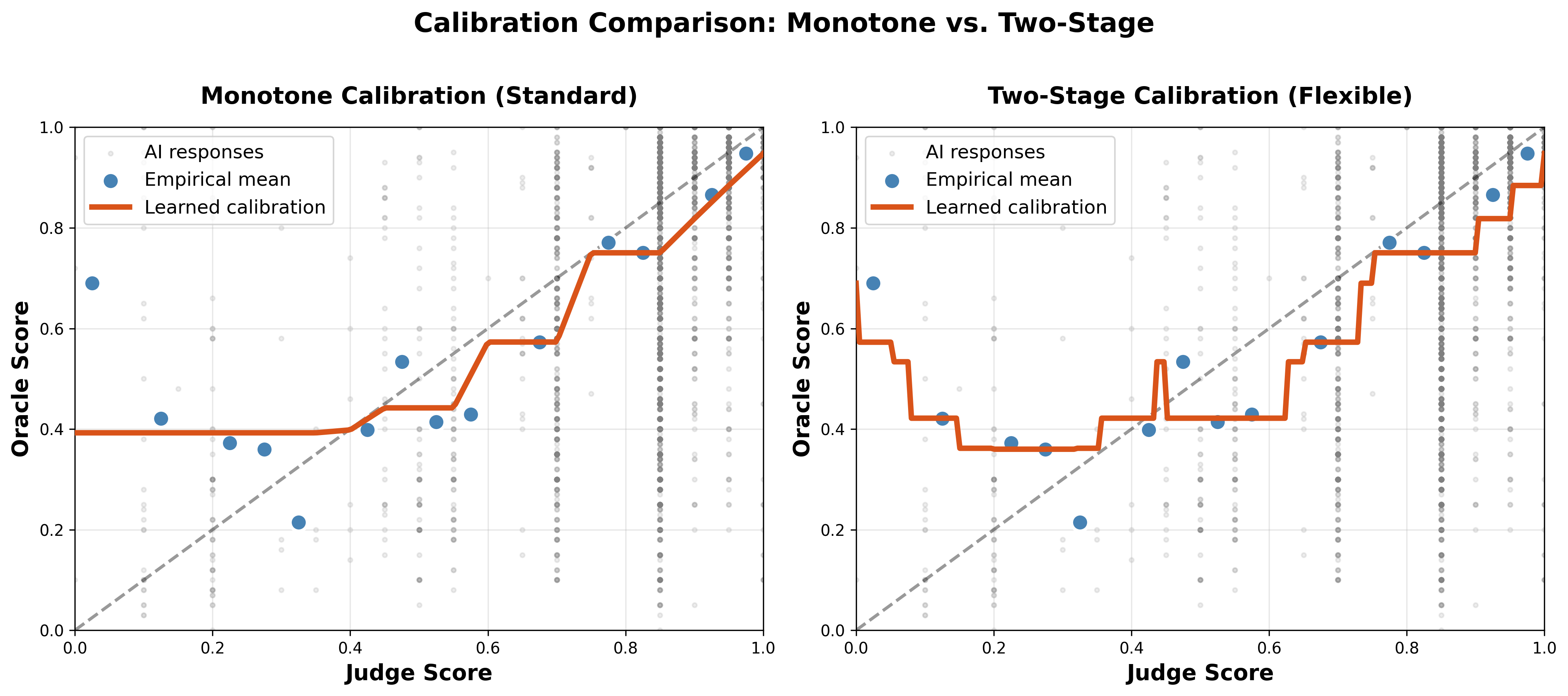
Click to enlarge • Calibration Comparison: Monotone (left) vs. Two-Stage (right)
The problem: Standard monotone calibration (left panel) forces a monotone fit even when judge scores don't strictly increase with quality. Notice how the red curve must increase everywhere, missing some low points. Two-stage calibration (right panel) fits the data better—both approaches produce valid calibration, but two-stage captures the true relationship more accurately when judge bias is present.
How two-stage works: Breaking down the bias
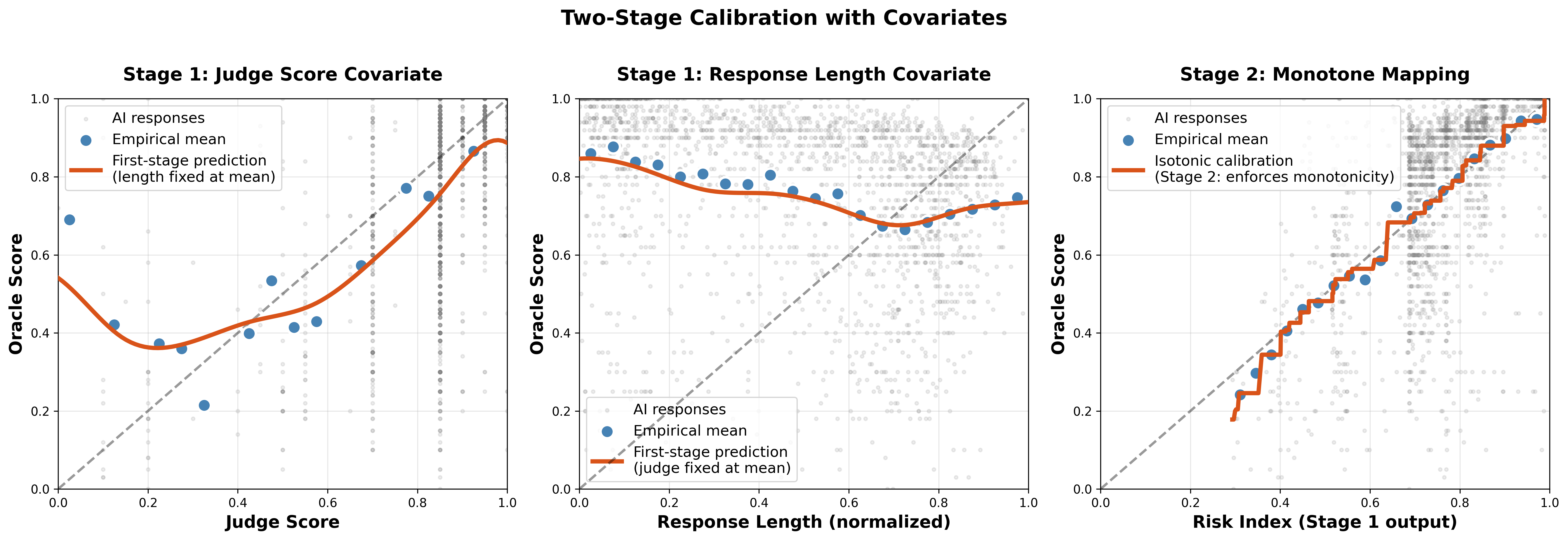
Click to enlarge • Two-Stage Process: Judge Score Covariate, Response Length Covariate, Final Monotone Mapping
Stage 1 (left two panels): Learn a smooth risk index T = g(S, response_length) using a spline. Left panel shows judge scores alone have a U-shaped relationship with quality (non-monotone). Middle panel reveals the culprit—judges reward verbosity even when quality plateaus or declines. The risk index combines both signals.
Stage 2 (right panel): Apply isotonic regression to the risk index T. The final calibration f(S, X) is monotone in T, mean-preserving (E[f] = E[Y]), and corrects for judge bias. Works with just 5–10% oracle coverage.
Why isotonic regression?
Isotonic regression is the default choice for learning because it imposes exactly the right inductive bias while making minimal assumptions:
- Minimal structural assumption: Only requires that higher judge scores → no worse oracle outcomes in expectation. Doesn't assume linearity, sigmoid shape, or any rigid functional form.
- Mean preservation by enforcement: We fit isotonic regression under a mean-preserving constraint on the labeled slice (or re-center predictions), so on that slice. This ensures your oracle KPI stays on the right scale. Off-slice means can differ if the mapping doesn't transport perfectly.
- Small-label efficiency: Works reliably with just 5–10% oracle coverage (200-500 labeled samples in this experiment). The shape constraint prevents overfitting—can't create spurious non-monotone regions. Adaptive complexity naturally produces piecewise-constant regions when data supports them.
- Ranking-sane: Never inverts judge order. No "perverse" regions where higher S predicts lower Y. Output is human-readable step blocks that give actionable thresholds.
- Computationally efficient: O(n log n) via Pool Adjacent Violators (PAV) algorithm [9]. Fast enough to refit thousands of times for cross-validation and uncertainty quantification.
- Informativeness monotonicity: Blackwell's notion of informativeness [10] suggests that richer judges with more informative scores should improve efficiency—finer σ-fields weakly lower variance in decision problems. While not a formal variance theorem for this exact estimator, the principle supports using the best available judge.
When to use alternatives: Parametric calibration (Platt scaling [6], Beta calibration [7]) offers lower variance if you're confident about the link function shape and have abundant labels. Unconstrained methods (neural networks, GAMs) only make sense when monotonicity fails and you have thousands of oracle labels. For this experiment's typical regime (250-2,500 oracle labels), isotonic hits the sweet spot of stability and flexibility.
Mean-preservation scope: Isotonic preserves the (weighted) mean on the labeled calibration slice; off-sample means can differ unless the calibration mapping transports.
SIMCal-W: Weight Stabilization
Used only for off-policy methods (IPS, DR) [2,3] that reweight logged data from π₀ to estimate V(π′). Direct methods don't use importance weights because they evaluate on-policy—each policy generates responses to the same prompts, so there's no distribution shift to correct for.
Off-policy methods compute importance weights for each logged response, measuring how much more likely π′ would have been to generate that response compared to π₀. When these weights become extreme (e.g., π′ strongly prefers responses π₀ rarely generated), the estimate becomes unstable—dominated by a few observations with huge weights.
SIMCal-W [4] stabilizes these importance weights via stacked score-indexed monotone projection. The algorithm combines multiple candidate weight vectors to minimize influence function variance while enforcing effective sample size (ESS) and variance constraints. Builds on isotonic calibration methods for inverse propensity weights.
Algorithm:
- Build candidates: Create increasing/decreasing isotonic weight functions via isotonic regression on (S, w)
- Compute OOF influence functions: For each candidate, compute out-of-fold influence functions using K-fold cross-fitting
- Optimize mixture: Solve quadratic program subject to , where is the covariance of OOF influence functions
Key insight: By stacking both increasing and decreasing isotonic candidates, SIMCal avoids requiring the researcher to assert the direction of the monotone relationship between scores and weights. The quadratic program automatically selects the optimal mixture based on influence function variance.
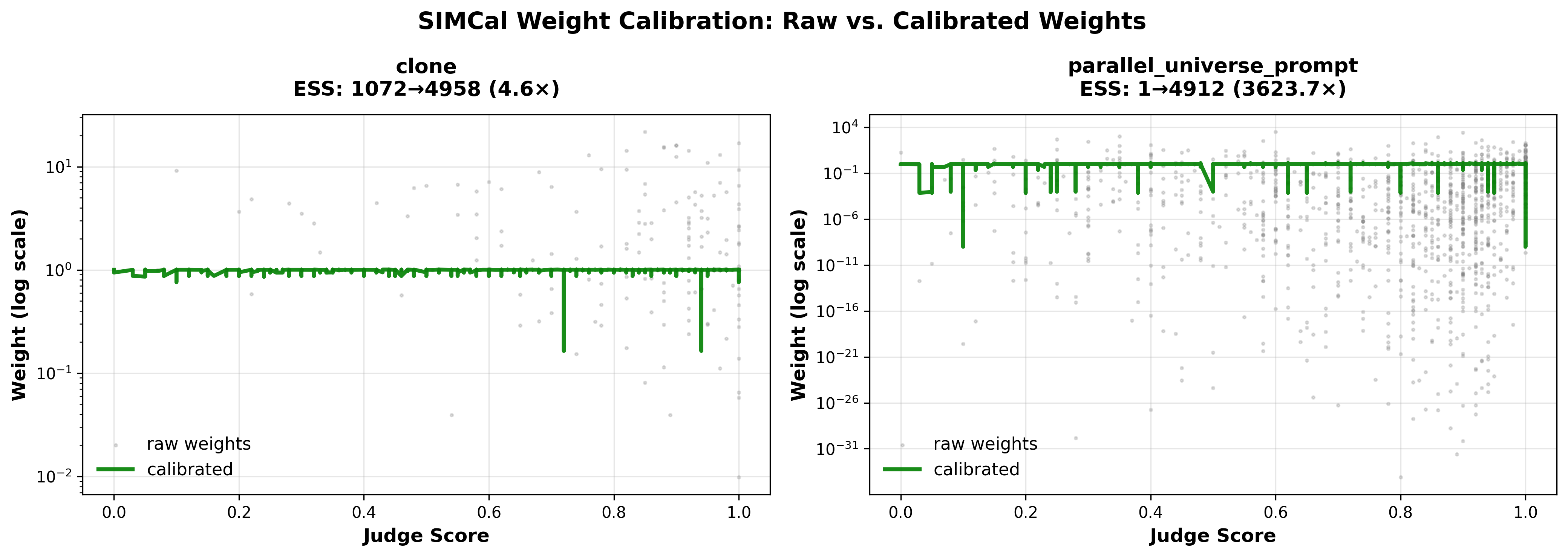
Click to enlarge • Weight Stabilization: Raw vs SIMCal-calibrated importance weights
Properties: Unit-mean on the logged distribution, nonnegative, and (S)-monotone; large ESS lifts (e.g., 0.4%→95%); improved balance within score strata. The mean-one isotonic projection reduces (L²) dispersion (ESS ↑) and typically improves Lorenz curves; it does not create overlap where none exists.
Connection to isotonic-calibrated IPW: SIMCal-W is an instance of the broader idea of calibrating inverse propensity weights via isotonic regression—projecting them onto a monotone, mean-preserving cone indexed by scores or covariates. This approach controls variance while preserving the estimand under stated assumptions, and it avoids the arbitrary cutoff choices required by traditional weight clipping. Recent causal inference results show this improves covariate balance and effective sample size compared to ad-hoc truncation methods. Note: We also explored policy-specific calibration (fitting separately for each policy), but it overfits with limited oracle data—future work will investigate hierarchical approaches that share information across policies while allowing some heterogeneity.
Terminology note: "Calibrated" in method names refers to weight calibration (SIMCal-W), not reward calibration. For example, "calibrated-ips" = SNIPS + SIMCal-W weights, but both SNIPS and calibrated-ips use AutoCal-R for rewards R = f(S, X).
Surrogate Model: What We Assume and How We Check It
Our calibration step relies on a surrogate sufficiency assumption (S1): after conditioning on the judge score (and selected covariates ), the oracle mean no longer depends on the raw output :
Intuition: the judge score (optionally with covariates like response length) is an information-rich summary of quality. The learned calibration function serves a similar role to the "surrogate index" proposed by Athey et al. [28], which combines multiple short-term proxies to predict a long-term outcome, though their work relies on stronger surrogacy assumptions and a two-sample data structure. Under this assumption and transportability of the mapping across policies (S2), AutoCal-R identifies using cheap scores, and our Direct/DR estimators are well-behaved.
The efficiency theory builds on Kallus & Mao (2024) [18], who derive semiparametric efficiency bounds for surrogate-assisted estimation under Missing At Random (MAR) oracle labeling—a weaker condition than surrogate sufficiency. Their framework doesn't assume S1, but provides the statistical foundation (cross-fitting, doubly robust estimation, OUA variance accounting) that CJE adapts when S1 does hold, enabling "calibrate once, evaluate everywhere" workflows.
When it's plausible
- Judge is strongly aligned with the oracle (monotone relationship).
- Known judge biases are captured by (e.g., response_length).
- Policies are "similar" (style shifts don't change ).
How we relax it
- Two-stage calibration learns a risk index , then applies monotone isotonic .
- DR estimators add an outcome model to correct residual bias.
- Richer judges or multi-judge stacking increase sufficiency.
When it fails
- Adversarial outputs with the same but different human value.
- Policy-specific style causing to shift.
- Out-of-range extrapolation (e.g., very low-quality unhelpful responses).
Diagnostics we run (oracle slice)
- Residual by policy/time: test (we report this transportability test; unhelpful fails).
- Stratified calibration: plot vs across bins of domain/length.
- Incremental signal: regress on and check if any extra features of (beyond ) add conditional signal—if yes, include them in .
Impact on estimators & uncertainty
- Direct: accurate if transports. Mis-specification mainly biases magnitudes; rankings often remain good if the mapping is monotone.
- DR: consistent if either stabilized weights are correct or the critic is correct, given correct reward calibration f. The "two chances" property protects against propensity vs. outcome model errors, but not against mis-calibrated f (S1 failure).
- SEs: OUA captures learning variance of but not structural bias if the surrogate assumption fails. We flag potential bias via residual tests; when flagged, treat CIs as optimistic for magnitude.
Practical tip: If residuals show structure by policy or domain, first add those covariates to ; if issues persist, calibrate per-policy or increase the judge's fidelity (multi-judge, richer features) before relying on magnitude estimates.
Assumptions Ledger: Quick Reference
Six core assumptions, how to test them, and what to do when they fail:
| Assumption | Applies To | Status | How to Test | Mitigation if Fails |
|---|---|---|---|---|
| A1 — Surrogate Sufficiency | All (Direct, IPS, DR) | ✅ Pass | Residuals flat by policy/domain; incremental signal tests | Add covariates to g(S,X); per-policy calibration; iterate on judge prompt; use richer judge |
| A2 — Transportability Surrogate→oracle mapping generalizes across policies and time | All (Direct, IPS, DR) | ✅ Pass except unhelpful | Mean residual = 0 by policy (Bonferroni); failure modes 1-3 | Recalibrate with small target slice; flag CI optimism |
| A3a — Score Coverage (Calibration) Oracle slice covers the support of | All (Direct, IPS, DR) | ✅ Strong except unhelpful | Overlay labeled vs. full score histograms; check tail bins | Stratified labeling on tail bins; active learning |
| A3b — Oracle Labeling MAR Subsampling independent of Y given (S,X) | All (Direct, IPS, DR) | ✅ Pass (uniform sampling) | Check if labeling rate varies with observed outcomes | Use uniform or S-stratified sampling; avoid outcome-dependent selection |
| A4 — Logging Policy Overlap Logger has support where target policies do | IPS, DR | ⚠️ Weak (ESS<1%) | ESS, tail index, max weight, CV diagnostics | SIMCal-W; fall back to DR/Direct; collect fresh draws |
| A5 — Propensity Validity Teacher-forcing yields valid π(A|X) | IPS, DR | ✅ Valid but noisy | Clone noise analysis; IPS failure despite SIMCal-W | Prefer Direct; if DR, rely more on critic than weights |
Estimator Requirements Matrix:
| Assumption | Direct | DR | IPS |
|---|---|---|---|
| A1 Surrogate sufficiency | ✓ | ✓ | ✓ |
| A2 Transportability | ✓ | ✓ | ✓ |
| A3a Score coverage | ✓ | ✓ | ✓ |
| A3b Oracle labeling MAR | ✓ | ✓ | ✓ |
| A4 Logging overlap | – | ✓ or correct critic | ✓ |
| A5 Propensity validity | – | ✓ or correct critic | ✓ |
Note: DR is "doubly robust"—requires either (A4+A5) or a correctly specified outcome model , conditional on correct reward calibration f (A1). The "two chances" protects against propensity vs. critic errors, not against S1 failure. Direct needs only A1–A3b. IPS requires all assumptions.
Connection to theory: These assumptions correspond to S1, S2, S3, L1, L2 in the technical appendix. A5 (propensity validity) is an LLM-specific operational concern within the general overlap framework.
Reward Calibration Failure Modes
Reward calibration learns a mapping from judge scores to oracle outcomes using labeled data from one policy or time period, then applies that mapping to new contexts. This transportability assumption can fail in three testable ways:
1. Policy-Specific Calibration
Failure mode: The mapping differs across policies. A judge score of 8 from Policy A might correspond to a different oracle value than a score of 8 from Policy B.
Why it happens: Policies have different output distributions—one might produce more verbose responses, use different vocabulary, or optimize for different judge signals. The same numeric score can reflect different underlying quality.
Observable signature: Within-policy rankings may remain accurate (judge scores correlate with quality within each policy), but cross-policy comparisons fail. If Policy A and Policy B have different true calibrations but you use a pooled , the relative ordering of policies can be wrong. Magnitude estimates are biased. Residuals show systematic patterns by policy rather than random scatter.
2. Extrapolation Beyond Calibration Range
Failure mode: A new policy's oracle values live outside the range covered by the calibration training data. For example, an adversarial policy might have oracle values below the minimum calibrated reward—even a judge score of 0 maps to a value higher than the true oracle outcome.
Why it happens: Calibration learns a monotone mapping from observed (S, Y) pairs. If a new policy produces responses that are worse than anything the calibrator has seen, the monotone constraint forces predictions to plateau at the training data minimum rather than extrapolate downward.
Observable signature: Ranking still works (relative ordering preserved), but point estimates are systematically biased upward for bad policies. Confidence intervals fail to cover the truth. Calibrated rewards show a floor effect—no predictions below the calibration training minimum.
3. Temporal Shift in Preferences
Failure mode: The mapping changes over time. User preferences drift—behaviors that were once valued become tiresome, or quality standards evolve. A calibration learned in January may be invalid by June.
Why it happens: Oracle labels reflect user preferences or business KPIs that evolve. Judge scores may be stable (judges consistently score verbosity as 8/10), but the mapping to oracle outcomes shifts (users who once liked verbose answers now prefer concise ones).
Observable signature: Calibration accuracy degrades over time. Recent validation data shows larger residuals than historical validation. Rankings can shift or reverse when preference changes alter the relative quality of different behaviors. For example, if users tire of verbosity, policies optimizing for conciseness may overtake verbose policies even though judge scores haven't changed. Recalibrating on recent data improves fit. Drift can be gradual (slow preference shift) or sudden (product changes, new user cohorts).
Calibration Transportability Test
Critical design choice: Given these potential failure modes, we designed the experiment to test whether calibration learned from one policy transports to others. The calibration function is learned using oracle labels only from the base policy, then applied to all 5 policies (base, clone, parallel_universe_prompt, premium, unhelpful). This tests a realistic deployment scenario: you calibrate your judge against oracle data from one configuration, then use that calibration to evaluate new variants.
Procedure:
- Sample oracle labels from
basepolicy only at the specified coverage rate (e.g., 10% = 499 labeled responses from base) - Learn calibration function using base policy data: where
- Apply the learned to all policies' judge scores to produce calibrated rewards: for all ~25k responses
- Estimate policy values for each of the 5 policies using the calibrated rewards
This directly tests failure modes #1 and #2. If the true mapping differs across policies (failure mode #1), using base-only calibration will introduce bias when estimating other policies. The experiment quantifies how severe this bias is in practice. For unhelpful specifically, we also test failure mode #2 (extrapolation): adversarial responses may produce oracle values below the calibration range learned from good policies, causing systematic underestimation. The statistical test reveals whether residuals are centered at zero (calibration transports) or show systematic bias (calibration fails).
Note: Failure mode #3 (temporal shift) is not tested here because both the oracle (GPT-5) and judge (GPT-4.1-nano) are frozen models evaluated on a fixed prompt set. There is no time dimension over which the S→Y relationship could drift. Testing temporal calibration stability would require re-evaluating policies at different time points or simulating preference changes.
Contrast with pooled calibration: An alternative design would pool oracle labels across all policies and learn a shared . This would improve calibration quality but wouldn't test real-world deployment constraints—you typically can't collect oracle data from the new variants you're trying to evaluate. Base-only calibration mirrors production reality.
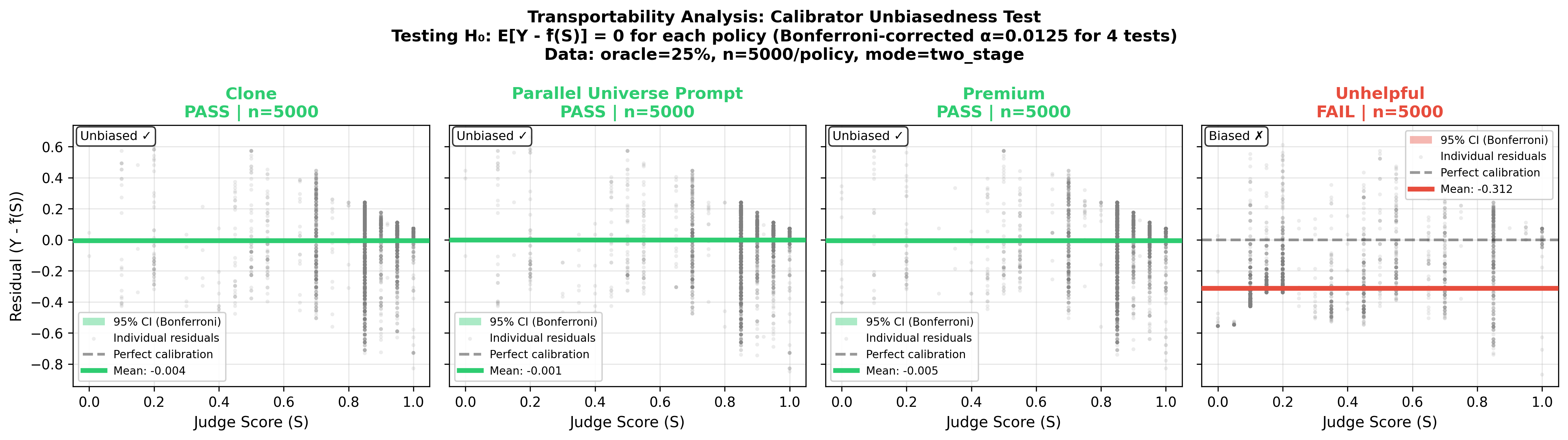
Click to enlarge • Calibrator transportability test at 25% oracle coverage. Testing H₀: E[Y - f(S, X)] = 0 for each policy (Bonferroni-corrected α=0.0125). Clone, Parallel Universe, and Premium pass (residuals centered at zero). Unhelpful fails (mean residual = -0.312), indicating the calibration function learned from base policy systematically underestimates oracle scores for adversarial responses.
Empirical Evidence from This Experiment
The transportability statistical test above directly tests failure mode #1 (policy-specific calibration). Results at 25% oracle coverage:
- ✓ Clone, Parallel Universe, Premium: Pass the unbiasedness test (mean residuals ≈ 0). Calibration learned from base policy successfully transports to these similar policies.
- ✗ Unhelpful: Fails the test (mean residual = -0.312, p < 0.0125 with Bonferroni correction). The calibrator systematically underestimates how bad these responses are. This indicates at least one of the failure modesis occurring—the test fails if either the S→Y mapping differs (mode #1) or responses fall below the calibration range (mode #2). Given the adversarial nature of the policy, mode #2 (extrapolation) is highly likely, though we cannot definitively determine from this test alone whether mode #1 is also contributing.
Practical implication: When evaluating adversarial or highly dissimilar policies, base-only calibration will be biased. Either collect oracle data from the new policy for recalibration, or use the residual patterns as a diagnostic signal that estimates may be unreliable.
Estimators
We compare 14 estimators across three families. Target: , where is the oracle outcome (GPT‑5 score normalized to [0,1]).
Why These Estimators? A Brief History
The three estimator families tested here sit on a long arc of statistical ideas. Importance weighting originates from survey sampling (Horvitz & Thompson, 1952), where you reweight observations to correct for unequal selection probabilities. The self-normalized variant (SNIPS, also called the Hájek estimator) stabilizes the ratio in practice and handles unknown normalizing constants—which is why it dominates in real applications despite being biased in finite samples.
Doubly robust methods give you "two chances"—if either your importance weights or your outcome model is correct, you get consistent estimates. This idea revolutionized causal inference in the 1990s and now underpins modern methods like Targeted Maximum Likelihood Estimation (TMLE).
CJE's SIMCal-W weight stabilization connects to recent work on isotonic-calibrated importance weighting: instead of arbitrarily clipping extreme weights, project them onto a calibrated, mean-preserving cone. This controls variance while preserving the estimand under stated assumptions—no ad-hoc cutoffs required.
Notation:
- : Oracle outcome (GPT‑5 score, ground truth)
- : Judge score (GPT‑4.1‑nano, cheap proxy)
- : Covariates (e.g., response_length, prompt_domain)
- : AutoCal-R calibration function mapping
- : Calibrated reward on oracle scale
- : Importance weight for off‑policy estimation
- : SIMCal-W stabilized importance weight
- : Outcome model (critic) predicting
1) Direct Model (DM)
Estimator:
Requires fresh draws from (on‑policy evaluation). Learns from oracle‑labeled subset.
- naive‑direct: (no calibration). Violates mean‑preservation.
- direct: learned via isotonic regression .
- direct+cov: Two‑stage: via spline, then isotonic .
Assumptions: Shared prompts (paired design), representative oracle sample, calibration transportability across , monotonicity in risk index .
2) Importance Sampling (IPS)
Primer: Teacher Forcing & Propensity Weights
Off-policy evaluation (OPE) tries to estimate how well a new policy π′ would perform using only data collected from an old logging policy π₀. This avoids the cost of generating fresh responses.
Propensity weights correct for the distribution shift: if π′ would have generated a different response than π₀ did, we reweight the logged outcome to account for this. When π′ strongly favors responses that π₀ rarely generated, weights become large and unstable.
Teacher forcing [11] is how we compute these propensities for text generation models. Given a logged response A (a sequence of tokens), we condition π′ on each prefix and ask: "what's the probability π′ assigns to the next token?" Multiply across all tokens to get . This requires the model to score arbitrary continuations, not just sample from its own distribution.
The problem: Most LLM APIs don't support teacher forcing reliably. Even when providers claim support, implementations can be non-deterministic or buggy. The CJE package provides a working implementation for Fireworks AI, but this remains a major deployment barrier for OPE in production.
Teacher forcing caveat: Even the clone policy (identical to base with different seed) shows non-deterministic behavior when teacher forcing logged responses. We analyzed the deviations and found them to be effectively random noise. This noise contributes to OPE failures but represents a real deployment challenge.
Deeper issue—structural validity: Recent theory shows that models trained with next-token prediction can learn "shortcut" predictors that don't reflect how the model would actually generate text. The token probabilities reported during teacher forcing might be systematically miscalibrated relative to the model's true generation distribution. This weakens the "two chances" guarantee of doubly robust methods when propensities come from teacher forcing—even a perfect outcome model can't save you if the weights are fundamentally wrong. Our results (IPS failure; DR requires SIMCal-W + strong critic) are consistent with this diagnosis.
Estimator: where from logged data under
Reweights logged data from to estimate . All variants use AutoCal‑R for rewards . Methods differ only in weight treatment:
- SNIPS: Raw self‑normalized importance weights (no SIMCal‑W).
- calibrated‑ips: SIMCal‑W stabilized weights via monotone projection on .
- +cov variants: Include response_length in both and propensity model.
Terminology note: SNIPS (self-normalized importance sampling) is the same as the Hájek estimator from survey sampling: . It's biased in finite samples but typically has lower variance than the unbiased Horvitz-Thompson estimator, and it handles unknown normalizing constants naturally—which is why it's the practical default in most applications.
Stability: . Low ESS indicates that the weights are dominated by a very small number of samples, making estimates unstable.
3) Doubly Robust (DR)
where predicts outcomes for logged actions under , and is computed via fresh draws from . Consistent if either or is correct. All variants use AutoCal‑R rewards and differ in weight treatment:
- dr‑cpo: Cross‑fitted with raw importance weights (no SIMCal‑W). (CPO = Cross-fitting with Pseudo-Outcomes)
- calibrated‑dr‑cpo: Cross‑fitted with SIMCal‑W stabilized weights .
- stacked‑dr: Optimal weighted combination of DR, TMLE, MRDR via influence functions (uses SIMCal‑W).
- tr‑cpo‑e: Triply robust with raw/Hájek weights (adds oracle label correction term, no SIMCal‑W). (TR-CPO-E = Triply Robust with Cross-fitting, Pseudo-Outcomes, and Efficient weighting)
Cross-Fitting & Orthogonality (how DR gets valid CIs)
- K=5 folds on
prompt_id(stable hash). Train nuisances on K−1 folds, predict on the held-out fold (OOF). - OOF predictions break dependence → Neyman-orthogonality in practice, so SEs/95% CIs are asymptotically valid.
- All DR variants here use cross-fitting (always on; not ablated). SIMCal-W uses an outer CV loop for honest weight calibration.
See Reproducing Results for fold plumbing details.
Cross-fitting gotchas
- Fold at prompt level to avoid leakage across samples of the same prompt.
- Use one fold scheme across calibrator, outcome model, and SIMCal outer CV.
- Very small oracle slices can make orthogonality tests noisy—interpret CI width, not just the point score.
Single-Turn vs. Multi-Turn (Agents)
This post evaluates single-turn responses, but CJE extends directly to agents / multi-turn settings. There are two practical patterns:
A) Terminal-Outcome
Score only the final output with a judge (), calibrate to oracle (), and evaluate as in the single-turn case. This minimizes labeling cost and keeps estimators unchanged.
B) Step-Weighted Trajectory
Score each step , calibrate step-wise, and aggregate a trajectory reward:
Choose to reflect your task: discounting, milestone weighting, or learned attributions.
Estimators: Direct methods use the same formulas, replacing single-turn rewards with . For OPE, sequential IPS multiplies per-step propensities; in practice this worsens degeneracy, so we recommend Direct or DR with a trajectory-level critic.
Oracle-Uncertainty Aware (OUA) Inference
Standard statistical practice treats learned nuisance functions (like our calibration function ) as if they were the true population function. This is approximately correct when the training sample is very large—but with oracle coverages of 5–50%, treating as fixed dramatically understates total uncertainty.
The Problem: Calibration Uncertainty
Consider estimating with the Direct Model: . The calibration function is learned from a small oracle slice (e.g., 250 labeled samples at 5% coverage). If we had a different oracle sample, we'd learn a different , which would produce a different estimate .This variance is real and non-negligible—ignoring it produces confidence intervals that are far too narrow.
Concrete example: At n=1000 and 5% oracle coverage (50 labels), OUA variance contributes ~55% of total uncertainty. Standard methods report SE ≈ 0.014 (treating as fixed), but the true SE ≈ 0.033 when accounting for calibration uncertainty. The "95%" CI without OUA has actual coverage around 70%—it's not calibrated.
The Solution: Delete-One-Fold Jackknife
OUA uses a delete-one-fold jackknife [12] procedure to quantify calibration uncertainty. The oracle labels are partitioned into folds (default K=5 for cross-fitted calibrators). For each fold k=1,...,K:
- Refit the calibrator: Train using only oracle labels from folds . This produces a calibrator with approximately of the oracle data (e.g., 80% for K=5).
- Recompute the estimate: Apply to the evaluation data and compute the policy value . For DM this is . For IPS/DR, also recompute stabilized weights (since SIMCal-W depends on ) and outcome models (for DR).
- Accumulate jackknife variance: After K iterations, compute the jackknife estimate of :The correction adjusts for the delete-one-fold sampling scheme.
Key principle: OUA captures oracle-only uncertainty. It holds the evaluation log (the S values being calibrated) fixed and only refits the components that depend on the calibrator. This maintains statistical independence with the base sampling variance , allowing us to simply add the two variance components.
Theoretical Foundation
The necessity of accounting for calibration uncertainty (OUA) is formalized in semiparametric efficiency theory [18]. Kallus & Mao (2024), building on Double/Debiased Machine Learning principles [29], show how techniques like cross-fitting (used in CJE's DR estimators and calibration) and doubly robust scores allow for valid inference even when nuisance functions like the calibrator are estimated flexibly from limited oracle data. Our delete-one-fold jackknife procedure provides a practical and asymptotically valid way to estimate this crucial variance component, ensuring that reported confidence intervals have correct coverage even when oracle labels are sparse.
Total Uncertainty Formula
The final standard error combines base sampling uncertainty and oracle uncertainty:
where is the base variance from the influence function (for DM: cluster-robust variance accounting for within-prompt correlation; for IPS/DR: influence function variance from reweighting and outcome modeling).
Confidence intervals are formed using a t-critical value with Welch-Satterthwaite degrees of freedom [13,14] when clusters or oracle folds are small (combines df from both variance components), falling back to normal quantiles for large samples. We report 95% CIs accounting for both sampling and calibration uncertainty. For general statistical guidance on eval reporting and paired inference, see Miller (2024).[27]
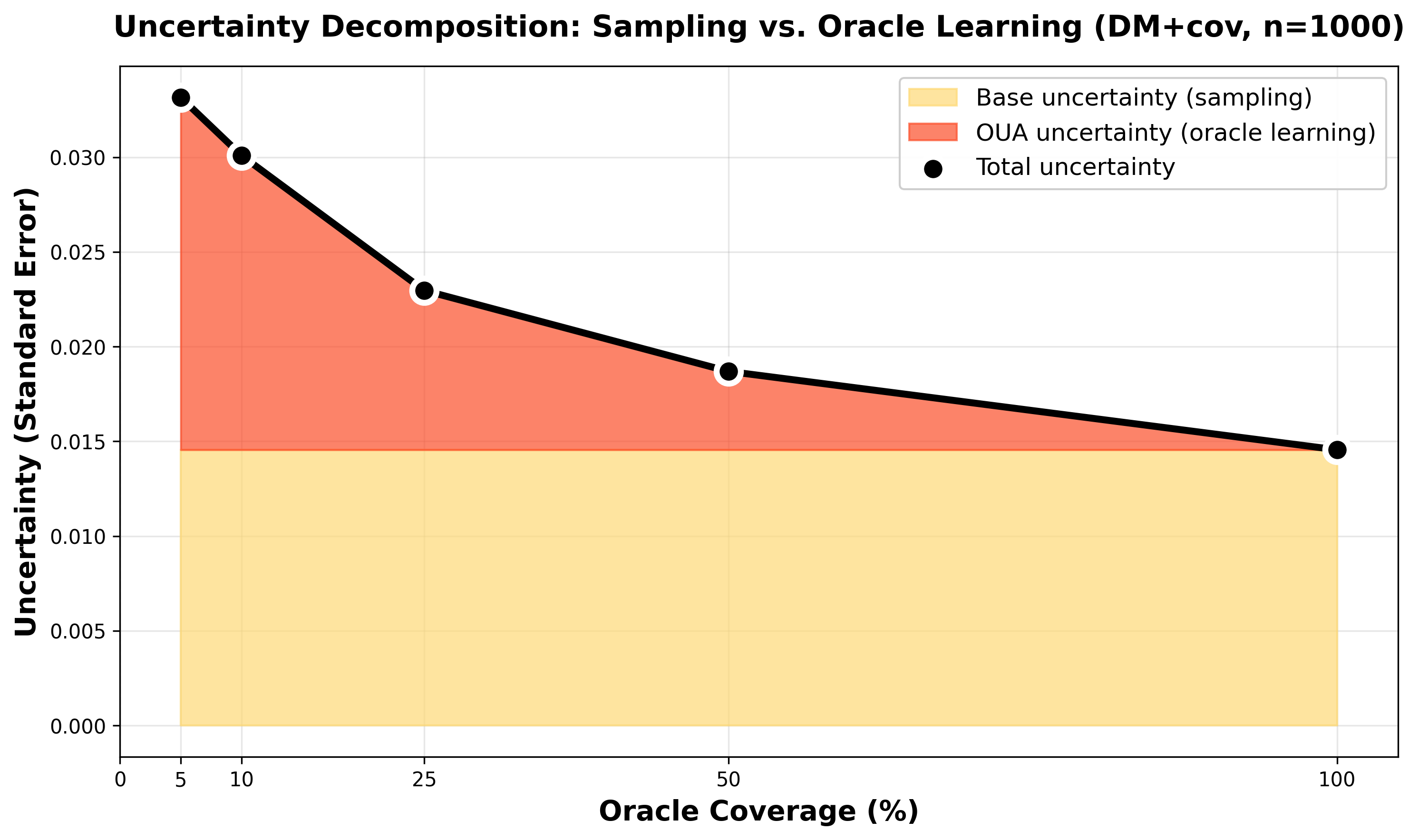
Variance decomposition at n=1000 for direct+cov. Blue: base sampling uncertainty (constant ~0.014). Orange: oracle uncertainty (dominates at 5% coverage ~0.018, vanishes at 100%). Total SE (black) drops from 0.033 to 0.015.
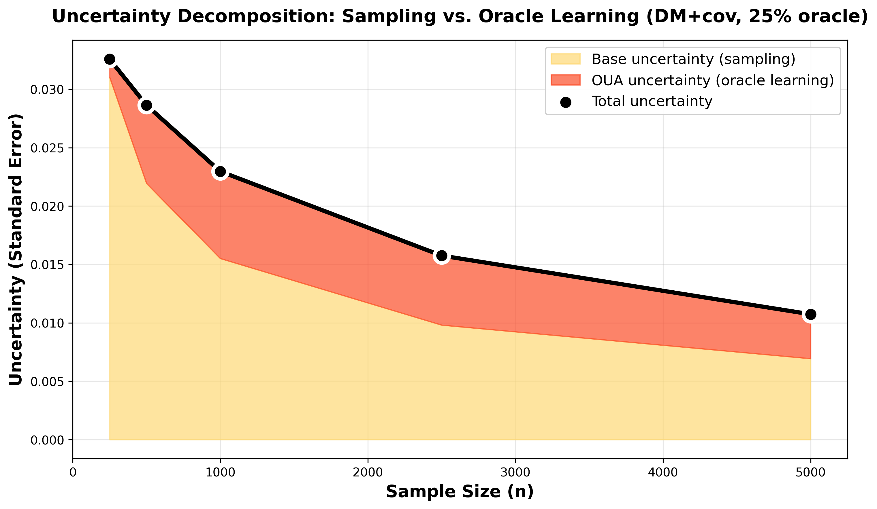
Variance decomposition at 25% oracle coverage for direct+cov across sample sizes. Blue: base sampling uncertainty (decreases with n). Orange: oracle learning uncertainty (also decreases with n, but slower). At small samples (n=200), oracle uncertainty dominates; at large samples (n=5000), both components matter. This shows you need to scale both the evaluation set and oracle labels.
When OUA is Skipped
OUA is automatically skipped at 100% oracle coverage. When every evaluation sample has a ground-truth label, there's no calibration step—we directly average the oracle outcomes. Since isn't learned, there's no calibration uncertainty to account for. The CJE package detects this and sets .
OUA share diagnostic: The fraction tells you whether label scarcity or prompt scarcity is the bottleneck. If OUA share > 50%, adding more prompts won't help—you need more oracle labels. If OUA share < 20%, you have sufficient labels and should focus on prompt coverage. This experiment reports OUA share for all estimators at every oracle coverage level.
Standard Errors with Agents & Human Oracles
With multi-turn agents, treat each conversation/trajectory as a cluster. Compute trajectory rewards (terminal or step-weighted) and use cluster-robust IF variance:
where indexes conversations, are influence-function contributions aggregated within a trajectory, and is the number of trajectories.
OUA proceeds as before but refits calibrators on delete-one-fold oracle slices and recomputes . With human oracles, add a rater component:
We combine degrees of freedom via Satterthwaite:
with (clusters), oracle folds, and raters.
Recommendation: For agents, prefer Direct (on a shared conversation set) or DR with a trajectory-level critic. If you must do OPE, use per-step DR with stabilized weights and monitor overlap diagnostics—sequential IPS alone typically degenerates.
Evaluation Metrics
For each estimator we report:
Note: All metrics below are computed excluding the unhelpful policy(an adversarial outlier that failed the transportability test—we knew base-only calibration wouldn't work for it). This exclusion doesn't materially affect findings.
- RMSEd (oracle-noise-debiased RMSE): Root mean squared error with oracle measurement noise removed. Computed as . This isolates estimator error from oracle label noise. Lower is better.
- IS (interval score) [15]: Winkler score for evaluating predictive intervals—penalizes both interval width and miscoverage. Lower is better. Combines calibration (does the 95% CI actually contain the truth?) and sharpness (how narrow is the interval?).
- Coverage %: Fraction of 95% CIs covering the truth (~95% is ideal)
- SE GM: Geometric mean of standard errors (lower = tighter)
- Pairwise %: Correct binary policy orderings (higher is better)
- Top‑1 %: Correctly identifies the best policy (higher is better)
- (Kendall's tau) [8]: Rank correlation (−1 to 1, higher is better)
- Runtime (s): Wall‑clock runtime
Standard Errors and Confidence Intervals
CJE provides complete uncertainty quantification accounting for all sources of variance, not just sampling uncertainty. Standard errors include three components:
- Influence function (IF) variance: Base sampling uncertainty from the data
- Monte Carlo (MC) variance: Additional uncertainty from finite fresh draws in DR estimators (in this experiment: 1 fresh draw per prompt per policy)
- Oracle uncertainty (OUA): Uncertainty from learning the calibration function with partial oracle coverage (see OUA section for full details)
Cluster-robust inference for paired designs: Direct methods cluster standard errors by prompt_id rather than treating all ~25k responses as independent. Since all 5 policies respond to the same 5k prompts, there are only 5k independent clusters. This accounts for within-prompt correlation and prevents underestimated standard errors.
Why this matters: The 85–99% coverage rates you'll see in the results are honest—they account for calibration uncertainty (OUA), clustering, and finite sample corrections (t-distribution). This is what makes CJE confidence intervals reliable for decision-making, not just optimistic point estimates.
Results
Metrics are averaged across all experimental regimes: 5 oracle coverages (5%, 10%, 25%, 50%, 100%), 5 sample sizes (250, 500, 1K, 2.5K, 5K), and 50 random seeds. This tests robustness to oracle availability and sample size.
Ablation Dimensions
1. Weight Calibration (Off-Policy Methods Only)
- Without SIMCal-W: SNIPS, dr-cpo use raw importance weights
- With SIMCal-W: calibrated-ips, calibrated-dr-cpo, stacked-dr use stabilized weights via isotonic projection
- Impact: SIMCal-W prevents weight degeneracy. Compare SNIPS (τ=−0.24) vs calibrated-ips (τ=−0.06), or dr-cpo (τ=0.57) vs calibrated-dr-cpo (τ=0.82)
2. Two-Stage Reward Calibration (+cov variants)
- Without +cov: Monotone calibration (direct, calibrated-ips, dr-cpo, etc.)
- With +cov: Two-stage calibration (direct+cov, calibrated-ips+cov, etc.)
- Impact: Adding response_length as a covariate handles judge bias toward longer responses. Improves direct methods (τ: 0.836 → 0.887), mixed impact on OPE where propensity modeling complexity increases
| Estimator | RMSEd | IS | Coverage % | SE GM | Pairwise % | Top‑1 % | τ |
|---|---|---|---|---|---|---|---|
| naive‑direct | 0.0828 | 2.9580 | 0.0 | 0.0039 | 90.9 | 79.6 | 0.817 |
| direct | 0.0225 | 0.0566 | 85.7 | 0.0072 | 91.8 | 84.1 | 0.836 |
| direct+cov | 0.0256 | 0.0582 | 87.0 | 0.0077 | 94.3 | 89.4 | 0.887 |
| SNIPS | 0.1596 | 0.7379 | 98.3 | 0.1815 | 38.3 | 8.7 | -0.235 |
| SNIPS+cov | 0.1842 | 0.7544 | 97.8 | 0.1842 | 37.4 | 6.4 | -0.252 |
| calibrated‑ips | 0.0246 | 0.5727 | 99.1 | 0.0963 | 47.1 | 19.1 | -0.058 |
| calibrated‑ips+cov | 0.0262 | 0.6084 | 99.2 | 0.1027 | 46.5 | 20.6 | -0.069 |
| dr‑cpo | 0.0460 | 0.2205 | 99.2 | 0.0371 | 78.4 | 46.3 | 0.567 |
| dr‑cpo+cov | 0.0570 | 0.2657 | 99.4 | 0.0449 | 79.1 | 50.1 | 0.581 |
| calibrated‑dr‑cpo | 0.0227 | 0.1359 | 99.5 | 0.0231 | 91.0 | 81.0 | 0.819 |
| calibrated‑dr‑cpo+cov | 0.0260 | 0.1399 | 99.3 | 0.0236 | 94.1 | 87.5 | 0.881 |
| stacked‑dr | 0.0226 | 0.0792 | 95.5 | 0.0125 | 91.9 | 83.1 | 0.837 |
| stacked‑dr+cov | 0.0281 | 0.0806 | 96.1 | 0.0128 | 92.1 | 84.7 | 0.842 |
| tr‑cpo‑e | 0.1355 | 0.1472 | 95.0 | 0.0341 | 72.4 | 32.9 | 0.448 |
| tr‑cpo‑e+cov | 0.0985 | 0.1491 | 94.6 | 0.0344 | 76.1 | 42.9 | 0.522 |
Legend: Green highlights best‑in‑column among the shown rows. Red flags failure modes.
Performance Across Regimes
Results vary substantially by sample size and oracle coverage. We define four quadrants and show direct+cov performance across them:
| Regime | Conditions | RMSEd | IS | Coverage % | Pairwise % | Top‑1 % | τ |
|---|---|---|---|---|---|---|---|
| Large-n, High-cov | n ≥ 2.5K, oracle ≥ 25% | 0.0039 | 0.0218 | 88.0 | 99.8 | 100.0 | 0.997 |
| Large-n, Low-cov | n ≥ 2.5K, oracle ≤ 10% | 0.0134 | 0.0572 | 75.2 | 99.0 | 98.5 | 0.980 |
| Small-n, High-cov | n ≤ 500, oracle ≥ 25% | 0.0219 | 0.0858 | 87.5 | 90.8 | 81.5 | 0.817 |
| Small-n, Low-cov | n ≤ 500, oracle ≤ 10% | 0.0540 | 0.2306 | 84.2 | 84.8 | 70.5 | 0.700 |
Key insight: Ranking accuracy degrades gracefully, but coverage suffers with low oracle availability. Even in the worst case (small-n, low-cov), direct+cov achieves 84.8% pairwise accuracy and τ = 0.700. With adequate sample size (n ≥ 2.5K), ranking remains excellent (≥98.5% top‑1) even at low oracle coverage, but coverage drops to 75.2% (target: 95%).
Statistical Power and Sample Size Planning
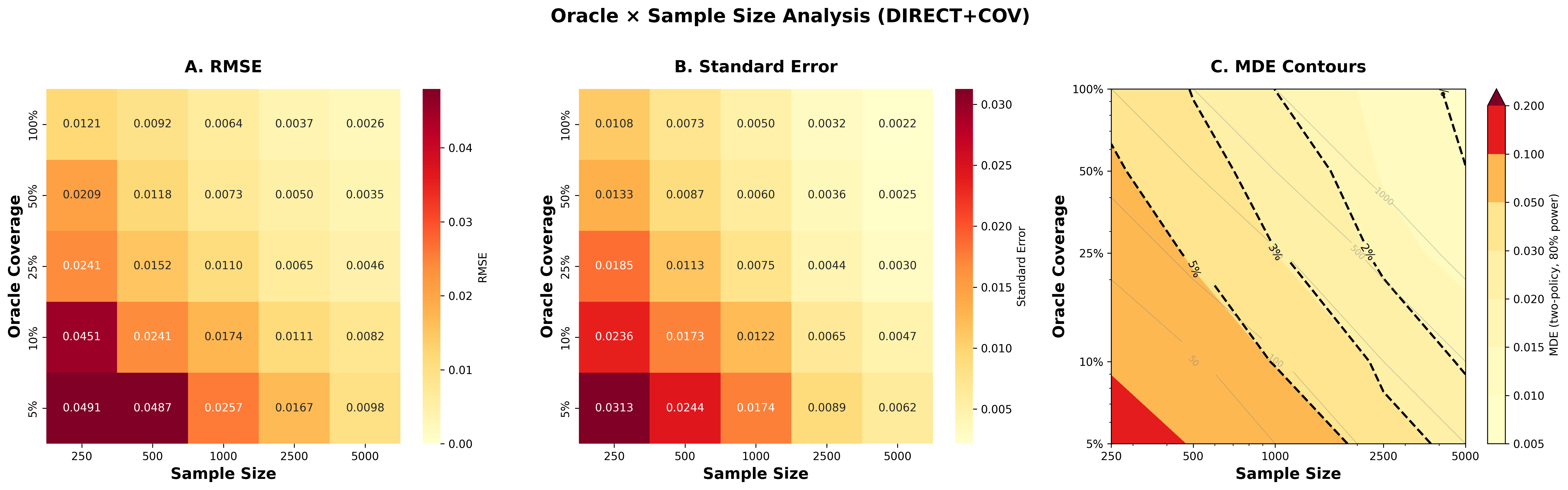
The heatmaps below show how accuracy (RMSE), precision (standard error), and statistical power (MDE) vary continuously with sample size and oracle coverage for direct+cov:
Click image to open full size in new tab
Panel A: RMSE improves dramatically with both sample size and oracle coverage (from 0.049 at n=250, 5% oracle to 0.003 at n=5K, 100% oracle). Panel B: Standard errors follow similar pattern, enabling tighter confidence intervals with more data. Panel C: MDE contours show statistical power—at n=1000 with 25% oracle coverage, you can reliably detect policy differences of ~2%. The 1% contour line shows the oracle/sample size combinations needed to detect small effects.
Practical takeaway: For ranking policies (not just detecting differences), n ≥ 1000 with 10–25% oracle coverage suffices. For detecting small effects (<1%), you need n ≥ 2.5K with ≥25% oracle coverage. Oracle coverage affects precision more than accuracy—you can rank well with limited oracle data, but need more for tight statistical guarantees.
Domain-Specific Calibration Recommended
The MDE and sample size recommendations shown here are specific to the Arena prompt distribution, GPT-4.1-nano judge, and GPT-5 oracle. Your domain may have different judge-oracle correlation, response variance, and effect sizes.
Best practice: Run your first analysis with more oracle coverage than you think you need (e.g., 50–100% if feasible). Use the diagnostics and uncertainty decomposition to empirically determine the minimum oracle coverage and sample size required for your precision targets. This calibration phase establishes your optimal design before scaling to production evaluation pipelines.
Analysis
1) Off-policy IPS fails catastrophically with teacher forcing
SNIPS fails to rank policies: Top-1 = 8.7% (random = 20%), τ = −0.235, Pairwise = 38.3%. This is worse than random guessing for policy selection.
Root cause: teacher forcing propensity estimation. Computing importance weights requires scoring each logged response under both the logging policy π₀ and target policy π′. For text generation, this means conditioning each policy on every token prefix and multiplying probabilities across the sequence. Even the clone policy (identical to base with different seed) shows propensity estimation noise due to non-deterministic teacher forcing implementations. When policies differ in model size, temperature, or system prompts, the distribution shift becomes severe.
Weight degeneracy: ESS collapses to 0.4–26.2% across policies (averaging 6.8%). Empirically, max(w)/median(w) > 10³ for most policies—a few extreme weights dominate the estimate, making it unstable regardless of sample size.
2) SIMCal-W boosts ESS up to 200×, but overlap remains scarce
Applying SIMCal-W weight stabilization to raw importance weights improves ESS dramatically and reduces weight concentration across multiple diagnostics:
| Policy | ESS (%) | Weight CV | Max Weight | Tail α | ||||
|---|---|---|---|---|---|---|---|---|
| SNIPS→Cal | Δ | SNIPS→Cal | Δ | SNIPS→Cal | Δ | SNIPS→Cal | Δ | |
| clone | 26.2→99.0 | +278% | 1.8→0.1 | +97% | 0.040→0.002 | +95% | 1.08→>10 | >900% |
| parallel_universe_prompt | 0.6→95.4 | +16k% | 26.6→0.2 | +99% | 0.617→0.003 | +100% | 0.56→>10 | >900% |
| premium | 0.7→82.1 | +12k% | 16.8→0.4 | +97% | 0.409→0.004 | +99% | 0.32→>10 | >900% |
| unhelpful | 0.4→84.6 | +22k% | 24.1→0.4 | +98% | 0.619→0.004 | +99% | 0.13→>10 | >900% |
ESS [16] (effective sample size) measures what fraction of the data contributes meaningfully to the estimate.Weight CV (coefficient of variation) measures weight concentration—lower is better.Max Weight shows the largest single importance weight—lower means less reliance on extreme observations.Tail α (Hill estimator) measures tail heaviness—higher values (>10) indicate lighter, more stable tails. SIMCal-W achieves 97-100% improvements across all diagnostics, yet IPS ranking still fails due to lack of overlap.
But IPS ranking still fails: Despite the ESS improvement, calibrated-ips achieves only 19.1% top-1 accuracy and τ = −0.058. The fundamental problem is lack of overlap between π₀ and π′—when the logging policy rarely generates responses similar to what the target policy would produce, no amount of weight stabilization can recover reliable estimates. SIMCal-W prevents numerical degeneracy but cannot create overlap where none exists.
Practical guidance on ESS: When reporting IPS or DR results, always include effective sample size. If ESS < 10 or ESS/n < 0.05, treat the estimate as unreliable—high variance and sensitivity to a few extreme weights make the point estimate and confidence intervals untrustworthy. In this experiment, raw SNIPS has ESS = 20 (0.4% of n=5000), which explains its random ranking performance.
Theoretical explanation: High ESS measures weight concentration but doesn't guarantee that the logger has meaningful coverage in target-typical regions—where the target policy concentrates its probability mass. See Coverage-Limited Efficiency for a formal treatment of the precision floor that no logs-only estimator can beat.
Implication for practice
Pure IPS requires substantial overlap between logger and target policies. With different LLM configurations (model size, temperature, system prompts), importance ratios become degenerate even after stabilization. This is a fundamental limitation of the logged data, not a solvable variance-reduction problem.
3) Doubly Robust + SIMCal-W recovers strong performance
DR estimators combine importance weighting with outcome modeling, providing consistency if either the weights or the outcome model is correct. With SIMCal-W weight stabilization, DR methods achieve performance comparable to direct methods:
- calibrated-dr-cpo+cov: Pairwise 94.1%, Top-1 87.5%, τ = 0.881, RMSEd = 0.026 — essentially matches direct+cov (94.3% pairwise, 89.4% top-1, τ = 0.887)
- stacked-dr: Best CI tightness (IS = 0.0792) with strong ranking (Pairwise 91.9%, τ = 0.837)
- dr-cpo (raw weights, no SIMCal-W): Top-1 drops to 46.3%, showing that weight stabilization is critical for DR to work
Why DR succeeds where IPS fails: The outcome model learns to predict oracle values from judge scores and covariates. Even when importance weights are unreliable due to poor overlap, the outcome model provides a baseline prediction. The weights only need to correct residual bias, not carry the entire estimation burden. SIMCal-W stabilizes these residual corrections.
Tradeoff: calibrated-dr-cpo+cov runs in ~20 s vs ~2.9 s for direct+cov (≈7× slower) due to cross-fitting and teacher forcing propensity estimation.
4) Direct Model is the practical winner
direct+cov achieves the best ranking performance with minimal computational overhead:
- Pairwise accuracy: 94.3%
- Top-1 accuracy: 89.4%
- Kendall's τ: 0.887
- Runtime: 2.9 s (7× faster than calibrated-dr-cpo+cov)
Why Direct dominates here: Part of the reason is that within-policy calibration (the first-stage isotonic fit) learns policy-specific biases in how the judge scores each policy's outputs. IPS and DR methods use pooled calibration across all policies, which can miss these policy-specific patterns.
Key advantage: no teacher forcing required. DM generates fresh responses from each policy on a shared prompt set, then scores them with the cheap judge. You never need to compute for arbitrary logged responses—avoiding the entire teacher forcing implementation challenge. This makes DM dramatically simpler to deploy in production.
Requirements: Shared prompts (paired design) and ability to generate responses from each candidate policy. When this is feasible—which it is for most LLM evaluation scenarios—DM should be your default.
5) Calibration is non-negotiable
naive-direct has 0% CI coverage, even though τ is 0.817. Without calibration, judge scores are on an arbitrary scale that doesn't match oracle outcomes. The rankings may be roughly correct, but the point estimates and confidence intervals are meaningless.
Calibrating the judge (direct) restores coverage to 85.7% and reduces RMSEd from 0.0828 → 0.0225 (73% reduction). Ranking also improves: top-1 accuracy increases from 79.6% → 84.1%, pairwise accuracy from 90.9% → 91.8%, and Kendall's τ from 0.817 → 0.836. Even for pure ranking tasks, reward calibration helps by correcting for systematic judge bias and learning the true relationship between judge scores and oracle outcomes.
AutoCal-R learns the monotone mapping from judge scores to oracle scale using just 5–25% oracle coverage, making estimates interpretable and CIs valid.
6) Covariates improve ranking across all methods
Adding response_length as a reward calibration covariate in the two-stage calibration consistently improves ranking performance. Comparing methods with vs without +cov:
- direct: Top-1 84.1%, τ = 0.836 → direct+cov: Top-1 89.4%, τ = 0.887 (+5.3 pp, +0.051)
- calibrated-dr-cpo: Top-1 81.0%, τ = 0.819 → +cov: Top-1 87.5%, τ = 0.881 (+6.5 pp, +0.062)
- stacked-dr: Top-1 83.1%, τ = 0.837 → +cov: Top-1 84.7%, τ = 0.842 (+1.6 pp, +0.005)
Why it works: Judges often reward verbosity even when longer responses don't provide more value. The two-stage calibration learns a risk index that captures this bias, then applies monotone calibration to the debiased index. This corrects systematic judge misalignment with oracle preferences.
Important: The response_length covariate enters only the reward calibration function f(S,X) to de-bias judge scores. It does not reweight toward longer or shorter outputs—its sole purpose is to learn and remove the systematic bias in how judges score responses of different lengths. The marginal distribution of response lengths remains unchanged.
Future work: Systematically discover additional bias-correcting covariates like prompt domain, difficulty, user context, or response structure.
7) Triply robust underperforms
tr-cpo-e underperforms here (Top-1 32.9%, RMSEd 0.136). The added complexity of a third robustness layer (oracle label correction) can introduce bias without careful tuning, especially when the underlying overlap assumptions are violated.
Methodological Takeaways
On‑policy DM should be your default
direct+cov offers the best ranking accuracy with low compute.
OPE requires overlap (and/or DR with a solid critic)
Use IPS only when policies are very similar (e.g., small temperature/top‑p changes). Otherwise prefer DR with calibrated rewards and cross‑fitted critics—understanding it still trails DM here and costs more.
Calibration and covariates matter
Calibration is required for valid CIs and better point estimates—and it also improves ranking. Adding response_length as a covariate improved ranking accuracy by 5–10 percentage points across methods. Future work: incorporating prompt domain, difficulty, and user context.
Limitations & Next Steps
What GPT-5-as-Oracle Tells Us — and What Generalizes to Humans
We use GPT-5 as the oracle here to stress-test estimators and uncertainty accounting. What does this say about CJE with human oracle labels?
- What carries over: The structure of CJE (calibrate a cheap judge to an oracle , then estimate with valid CIs) is unchanged. AutoCal-R's monotone/two-stage calibration and the OUA variance decomposition apply verbatim when the oracle is human.
- Where to be cautious: Model-as-oracle and model-as-judge can share biases, inflating alignment and ranking accuracy. With human oracles, noise and rater heterogeneity increase uncertainty; CIs widen appropriately when we account for that noise in OUA.
- Practical tactic: If your goal is human impact, calibrate against a small human slice and keep GPT-5 for scale. Compare residuals as a diagnostic; systematic drift indicates you should recalibrate on humans.
OUA with Human Oracles
When multiple raters label the oracle slice, treat the observed oracle as a noisy measurement of a latent target . Our standard error adds an extra component for rater noise:
In practice we estimate via the delete-one-fold jackknife over oracle folds (as in this paper), and by a lightweight delete-one-rater jackknife (or an item-level bootstrap if raters are sparse). Degrees of freedom combine by Satterthwaite as in our main OUA section.
External Validity: Generalizing to New User Populations
This experiment evaluates policies on Arena prompts. But what if you care about performance on a different user population—a new domain, geography, or user cohort? For example: your oracle labels come from expert raters (source distribution), but you need to estimate quality for general users (target distribution).
Doubly robust methods can handle this transport problem. Collect a small set of oracle labels from your source population and cheap judge scores from both source and target populations. The DR estimator requires two models: (1) an outcome model that predicts how oracle labels relate to judge scores (calibration), and (2) a density ratio model that reweights source data to match the target population.
The estimator is consistent if either model is correct. If your calibration function f(S,X) transports well (the relationship between judge scores and oracle outcomes is the same in both populations), you don't need perfect density ratio estimates. Conversely, if you have good density ratios but imperfect calibration, you still get valid estimates.
Practical use case: You have human preference data from a pilot study (source) but need to evaluate system performance for production users (target). Use DR with source oracle labels + target LLM-judge scores + a simple covariate-based density ratio model. We plan a follow-up Arena-style study demonstrating this design for domain transport.
Temporal Dynamics: When Preferences Drift Over Time
Judge scores reflect preferences at a point in time, but user preferences can drift. What users love in Week 1 may annoy them by Week 4—yet if your judge was trained on old data, it won't capture this shift. The result: your judge-to-oracle calibration breaks silently, and estimates become unreliable.
Real Example: Claude Sycophancy
Users initially enjoyed Claude's validating responses—"You're absolutely right!" felt supportive and engaging. But after extended use, many reported finding the sycophancy cloying and untrustworthy. When Claude validated obviously incorrect statements, users began questioning all its responses [HN discussion,GitHub issue].
The failure mode: A judge trained on initial user ratings would score sycophantic responses highly. But user preferences shifted—what was engaging became annoying. If you calibrated to oracle labels from January and evaluated policies in March, your estimates would be systematically biased. The judge-oracle mapping inverted.
How CJE handles temporal drift: Use the transportability test shown earlier in this post. Periodically collect fresh oracle labels on new batches and test whether your existing calibration function still produces unbiased predictions: . If residuals are systematically non-zero, your calibration has drifted. Re-calibrate with 200-500 fresh oracle labels from the current time period. The framework's modular design makes recalibration cheap—you don't need to retrain judges, just update the mapping from to using recent outcomes.
Design pattern for production: Collect oracle labels continuously (even if sparse—5-10% coverage is enough). Run the transportability test monthly on new batches. If it fails (Bonferroni-corrected p < 0.05 indicates systematic bias), you have two options:
- Re-calibrate: Update the mapping with fresh oracle labels (200-500 samples). This is fast and doesn't require retraining the judge. Works well when the judge's relative rankings are still good, but the mapping to oracle scale has shifted.
- Refine the judge: Manually inspect examples with the largest residuals . Look for systematic patterns (e.g., judge consistently underrates concise responses, or overrates verbose explanations). Update the judge prompt/template to fix these biases. This is more work but produces a better-aligned judge going forward.
For high-stakes decisions, pair this with A/A tests: evaluate your base policy against itself; if CJE detects a spurious difference, your calibration needs updating.
- Human-generated oracle labels: This experiment uses GPT-5 as the oracle, not real human preferences or business metrics. The most critical validation is replicating these results with actual human labels(crowdsourced preferences, expert annotations) and production KPIs (conversion rates, user retention, revenue, task completion). Model-based judges and oracles may share systematic biases that don't transfer to human judgments. Human preferences are noisier, more context-dependent, and exhibit different calibration relationships than LLM scores.
- Scope: Results reflect this prompt distribution and these policies. OPE stability depends on overlap; DM results are on‑policy to this eval set. Generalization to other domains (code generation, summarization, creative writing) requires domain-specific validation.
- SNIPS failure modes: Quantify minimum viable overlap (ESS targets; tail indices) for OPE viability. When is teacher forcing accurate enough for reliable propensity estimation?
- Oracle budget: How low can oracle coverage go while preserving calibration quality and ranking accuracy? Can we push below 5% with more sophisticated calibration methods or active learning for label allocation?
- Covariates: Systematic discovery beyond
response_length(prompt domain, difficulty, user context, response structure). Can we automatically identify bias-correcting covariates from data?
Try It Yourself: Working with the Data
To build intuition for how this works, let's look at the actual data structure and run a simple analysis. The CJE repository includes a 1k-sample slice of Arena data in examples/arena_sample/ for experimentation.
What the data looks like
Each logged sample contains the prompt, response, judge score, log probabilities, and (for a subset) oracle labels:
{
  "prompt": "What is the difference between OpenCL and CUDA?",
  "response": "OpenCL is an open standard maintained by Khronos...",
  "base_policy_logprob": -14.73,          // Log prob under logging policy
  "target_policy_logprobs": {             // Log probs for target policies
    "clone": -14.73,
    "parallel_universe_prompt": -18.25,
    "unhelpful": -42.12
  },
  "judge_score": 0.85,                    // Cheap judge score (0-1)
  "oracle_label": 0.86,                   // Ground truth (25% of samples)
  "metadata": {"prompt_id": "arena_1574"}
}
Fresh draws for each target policy include new responses generated at evaluation time:
{
  "prompt_id": "arena_0",
  "prompt": "What is the difference between OpenCL and CUDA?",
  "response": "OpenCL (Open Computing Language) and CUDA...",
  "judge_score": 0.85,
  "oracle_label": 0.86,    // 25-50% coverage for calibration
  "draw_idx": 0
}
Running the analysis
The experiments in this post use CJE's estimators with the data structure above. Here's how to run a similar analysis on the demo data:
from cje import analyze_dataset
from pathlib import Path

# Path to demo data (1k Arena samples)
data_dir = Path("examples/arena_sample")

# Direct Mode: use only fresh draws with oracle labels for calibration
results = analyze_dataset(
    fresh_draws_dir=str(data_dir / "fresh_draws"),
    include_response_length=True,  # Add response_length covariate
    verbose=True
)                                   # Auto-selects Direct Mode

# Results include estimates, standard errors, and confidence intervals
print(f"Policy estimates: {results.estimates}")
print(f"Standard errors: {results.standard_errors}")
print(f"95% CIs: {results.confidence_interval(alpha=0.05)}")

# DR Mode: combine logged data (IPS) with fresh draws (DM)
results_dr = analyze_dataset(
    logged_data_path=str(data_dir / "logged_data.jsonl"),
    fresh_draws_dir=str(data_dir / "fresh_draws"),
    verbose=True
)                                   # Auto-selects Doubly Robust
The estimator is automatically chosen based on the data you provide. You can override this by passing estimator="..." to select a specific variant (e.g., "stacked-dr" vs "calibrated-dr-cpo"). The function handles calibration, uncertainty quantification, and returns structured results with policy rankings and statistical tests. See the CJE repository's examples/ directory for complete worked examples including visualization code.
Citation
If you use this work, please cite:
BibTeX
@misc{landesberg2025arena,
  author = {Landesberg, Eddie},
  title = {Arena Experiment: Benchmarking 14 Estimators on 5k LLM Evaluations},
  year = {2025},
  month = {October},
  url = {https://cimolabs.com/blog/arena-experiment},
  note = {CIMO Labs Technical Report}
}
Plain Text
Landesberg, E. (2025). Arena Experiment: Benchmarking 14 Estimators on 5k LLM Evaluations. CIMO Labs Technical Report. https://cimolabs.com/blog/arena-experiment
References
Reproducing the Results
Data & Code Availability (Coming Soon)
The ablation study experiments were run using the cje-eval repository, which contains all experiment data, generated responses, oracle labels, and replication scripts (14 estimators × 13 configurations × 5 policies). We are working on making this repository public. This page will be updated with full replication instructions once cje-eval is released.
In the meantime, you can explore the CJE library and run your own experiments:
Cross-Fitting Implementation
DR estimators use cross-fitting to ensure valid inference. Here's how the fold plumbing works:
from cje.data.folds import get_folds_for_dataset
from cje.calibration import calibrate_dataset

fold_ids = get_folds_for_dataset(dataset, n_folds=5, seed=42)  # prompt_id-hash stable
calibrated, calres = calibrate_dataset(
    dataset,
    enable_cross_fit=True,   # default True
    n_folds=5,
    covariate_names=['response_length']
)
# DR estimators consume the OOF predictions tied to these folds.
The get_folds_for_dataset function assigns each prompt to exactly one fold using a stable hash, ensuring no leakage across fold boundaries. The calibrator trains on K−1 folds and predicts on the held-out fold, producing out-of-fold (OOF) predictions that break the dependence between nuisance estimates and the data used for inference.
Cite this work
APA
Eddie Landesberg. (2025, October 25). Arena Experiment: Benchmarking 14 Estimators on 5k LLM Evaluations. CIMO Labs Blog. https://cimolabs.com/blog/arena-experiment
BibTeX
@misc{landesberg2025arena,
  author = {Eddie Landesberg},
  title = {Arena Experiment: Benchmarking 14 Estimators on 5k LLM Evaluations},
  howpublished = {\url{https://cimolabs.com/blog/arena-experiment}},
  year = {2025},
  note = {CIMO Labs Blog}
}